Detecting Rest Stops in GPS Track Data

Problem Statement

Develop an algorithm that automatically classifies GPS track points as either "moving" or "stationary".

Nomenclature

$\tau_{i},i=0,\ldots,n$ List of time stamps in a GPS track.
$\boldsymbol{x}_{i},i=0,\ldots,n$ List of global position measurements corresponding to the time stamps $\tau_{i}$.
$T_{i}=\tau_{i}-\tau_{i-1},i=1,\ldots,n$ Time interval between successive measurements.
$S_{i}=d\left(\boldsymbol{x}_{i},\boldsymbol{x}_{i-1}\right),i=1,\ldots,n$ Distance between successive measurements.
$M_{i},i=1,\ldots,n$ Indicator of motion state of device in period before observation i. $M_{i}=1$ indicates device was moving. If $M_{i}=0$, it was stationary.
$\sigma_{\varepsilon}^{2}$ Device position measurement error variance, each dimension, m².
$\bar{v}$ Mean speed of device when moving, (m/sec).
$\sigma_{v}^{2}$ Variance of device speed when moving, (m/sec)².
$\mu_{0},\sigma_{0}^{2}$ Truncated normal distribution mean and variance parameters for time interval between measurements when device is at rest.
$\mu_{1},\sigma_{1}^{2}$ Truncated normal distribution mean and parameters for time interval between measurements when device is moving.

Summary

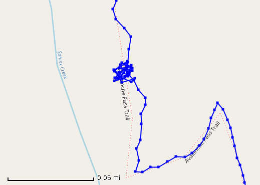
The picture at the right plots part of a track from one of my trips. Guess where the rest stop occurred! A cluster of track points forms around the point where we stopped. The track points vary from point to point due to GPS measurement error.

The problem is to find an algorithm that classifies all of the track points as either "stationary" or "moving". This has to be done in the presence of noise. This article is a summary of that project. It will propose a model for GPS speed measurements where the GPS device can be in one of two states: stationary or moving. It will describe how the unknown parameters of the model can be estimated by maximum likelihood estimation (MLE). It will show the results of the MLE algorithm for a track that was recorded during one of my summer trips.

Details of this project, including equations and Python scripts are in Likelihood function for GPS movement data (normal inter-measurement time distributions) and Convolution of a non-central chi-square with a central chi-square distribution. These documents are exports of the Jupyter notebooks that made the calculations.

A GPS track consists of time-stamped positions $\left(\tau_{i},\boldsymbol{x}_{i}\right),i=0,\ldots,n$. If we take successive differences on the times and positions, $T_{i}=\tau_{i}-\tau_{i-1}, S_{i}=d\left(\boldsymbol{x}_{i},\boldsymbol{x}_{i-1}\right)$, then we have series that can detect motion and even estimate speed. ($d\left(\boldsymbol{x},\boldsymbol{y}\right)$ is a function that computes the great circle distance between any to points on the Earth's surface.) When the device is moving, $S_{i}$ is the sum of the true distance moved during the time interval $T_{i}$ and the difference of two position measurement errors. When the device is stationary, $S_{i}$ contains only the difference in measurement errors and no movement distance.

The plot at right is a scatter diagram of one data set of successive differences from a backpack trip near Mount Brewer, CA. The device was a Garmin eTrex. We see that the eTrex sample interval varied from 1 to 42 seconds, but was typically every 15 seconds. We can see two modes in the scatter diagram. One is centered at 18 seconds and 15 meters between measurements.

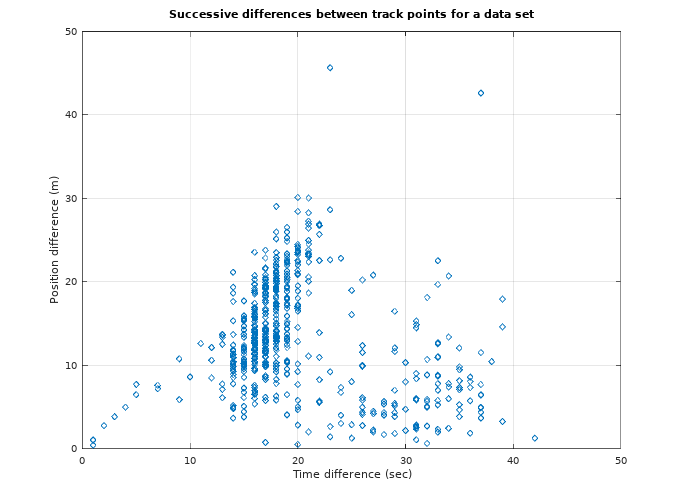
scatter diagram of successive differences

The other is centered around 30 seconds and 5 meters between measurements. The latter mode appears to be associated with the device in the stationary state, since the low position differences can be explained by measurement error.

For our purposes, a statistical model should describe two states: stationary and moving. It should describe the sources of errors in the observations $T_{i}, S_{i}$ in each state. Details of the model derivation are in the modeling paper. Here, I just summarize the model assumptions, the log-likelihood function and numerical results. The model assumptions are:

The device is either in a “stationary” or a “moving” state.
While in the stationary state, $S_{i}^{2}$ is entirely from GPS measurement error.
While in a the moving state, $S_{i}^{2}$ is the sum of GPS measurement error and a component from the movement speed.
Movement speed varies from measurement to measurement according to a normal distribution about a mean speed.
GPS measurement error has a two-dimensional Gaussian distribution with mean zero and variance $\sigma_{\varepsilon}^{2}$ in each dimension.
Regardless of the moving state of the device, the time interval between measurements varies as a normal distribution.
The mean of the time interval between measurements for the stationary state is greater than then mean for the moving device.
The variance of the time interval between measurements for the stationary state is no greater than the variance for the moving device.

The unknown parameters to be estimated are $M_{i},i=1,\ldots,n$, $\sigma_{\varepsilon}^{2}$, $\bar{v}$, $\sigma_{v}^{2}$, $\mu_{0},\sigma_{0}^{2}$, $\mu_{1},\sigma_{1}^{2}$ as defined under Nomenclature above. The most important of these parameters are the classifiers $M_{i},i=1,\ldots,n$. They classify each interval of the track as either moving ($M_{i}=1$) or stationary ($M_{i}=0$).

The derived formula for the log-likelihood function of the observations $T_{i}, S_{i}$ is:

$$L\left(\left\{ \left(T_{i},S_{i}^{2}\right)\right\} _{i=1}^{n}|\left\{ M_{i}\right\} _{i=1}^{n},\bar{v},\sigma_{v},\sigma_{\varepsilon}^{2}\right)$$ $$=\sum_{i=1}^{n}(1-M_{i})\left(-\log\left(1-\Phi\left(-\frac{\mu_{0}}{\sigma_{0}}\right)\right)-\frac{1}{2}\log\left(2\pi\sigma_{0}^{2}\right)-\frac{\left(T_{i}-\mu_{0}\right)^{2}}{2\sigma_{0}^{2}}-\log\left(2\sigma_{\varepsilon}^{2}\right)-\frac{S_{i}^{2}}{2\sigma_{\varepsilon}^{2}}\right)$$ $$+M_{i}\left(-\log\left(1-\Phi\left(-\frac{\mu_{1}}{\sigma_{1}}\right)\right)-\frac{1}{2}\log\left(2\pi\sigma_{1}^{2}\right)-\frac{\left(T_{i}-\mu_{1}\right)^{2}}{2\sigma_{1}^{2}}+\log\left(f_{M=1}\left(S_{i}^{2}|T_{i}\bar{v},T_{i}^{2}\sigma_{v}^{2},\sigma_{\varepsilon}^{2}\right)\right)\right)$$
where $f_{M=1}\left(S_{i}^{2}|T_{i}\bar{v},T_{i}^{2}\sigma_{v}^{2},\sigma_{\varepsilon}^{2}\right)$ is the density function of $S_{i}^{2}$ when the device is moving, the expression of which is a convolution:
$$f_{M=1}\left(S_{i}^{2}|T_{i}\bar{v},T_{i}^{2}\sigma_{v}^{2},\sigma_{\varepsilon}^{2}\right)=\frac{1}{2T_{i}^{2}\sigma_{v}^{2}\sigma_{\varepsilon}^{2}2^{\frac{1}{2}}\Gamma\left(\frac{1}{2}\right)}\int_{0}^{S_{i}^{2}}\left(\frac{S_{i}^{2}-y}{T_{i}^{2}\bar{v}^{2}}\right)^{-\frac{1}{4}}\left(\frac{y}{\sigma_{\varepsilon}^{2}}\right)^{-\frac{1}{2}}\exp\left(-\frac{1}{2}\left(\frac{S_{i}^{2}-y}{T_{i}^{2}\sigma_{v}^{2}}+\frac{\bar{v}^{2}}{\sigma_{v}^{2}}+\frac{y}{\sigma_{\varepsilon}^{2}}\right)\right)I_{-\frac{1}{2}}\left(\frac{\bar{v}}{T_{i}\sigma_{v}^{2}}\sqrt{S_{i}^{2}-y}\right)dy$$
The script $\textsf{f_non_central_convolved}$ (see Convolution of a non-central chi-square with a central chi-square distribution) evaluates $f_{M=1}\left(S_{i}^{2}|T_{i}\bar{v},T_{i}^{2}\sigma_{v}^{2},\sigma_{\varepsilon}^{2}\right)$ by numerical integration. The script $\textsf{f_llmovement}$ (see Likelihood function for GPS movement data (normal inter-measurement time distributions)) evaluates the log-likelihood function. Cell $\textsf{In [9]}$ under the heading Maximum Likelihood Estimation is a script that finds the maximum likelihood estimates for the unknown parameters.

For our example track, the maximum likelihood estimate of the classifiers $\hat{M}_{i},i=1,\ldots,n$ are shown in this scatter diagram. The value of $\hat{M}_{i}$ for each pair $(T_{i}, S_{i})$ is coded by color. The MLEs of the other parameters are:

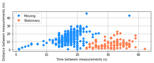$\hat{\sigma}_{\varepsilon}^{2} = 27.51$ m² ($\hat{\sigma}_{\varepsilon} = 5.25$ m)
$\hat{\bar{v}} = 0.831$ m/sec
$\hat{\sigma}_{v}^{2} = 0.122$ (m/sec)² ($\hat{\sigma}_{v} = 0.349$ m/sec)
$\hat{\mu}_{0} = 31.0$ sec
$\hat{\sigma}_{0}^{2} = 11.7$ sec² ($\hat{\sigma}_{0} = 3.42$ sec)
$\hat{\mu}_{1} = 17.1$ sec
$\hat{\sigma}_{1}^{2} = 11.7$ sec² ($\hat{\sigma}_{1} = 3.42$ sec)

The MLE algorithm behaved as expected. It classified those pairs with small distance intervals and long time intervals as rest stops, leaving the remaining pairs to form a reasonable regression of distance versus time. The mean speed of 0.831 m/sec (1.9 miles/hour) is consistent with my hiking speed from other trips. The variability of hiking speed, 0.349 m/sec or about 42% of the mean hiking speed is typical of varying conditions of this hike; the track includes level travel as well as climbing switchbacks. The GPS error of 5.25 m in each direction is about what I expect.

As a final check, we can plot the positions of the points that were classified as rest stops over a plot of the track. This plot appears at the right. I remember that the longest stops on that hiking day were at the trailhead near (100, -200) on the graph, at the bridge crossing of the South Fork near (2800, -800), and close to the Sphinx Trail junction near (3800, -1800).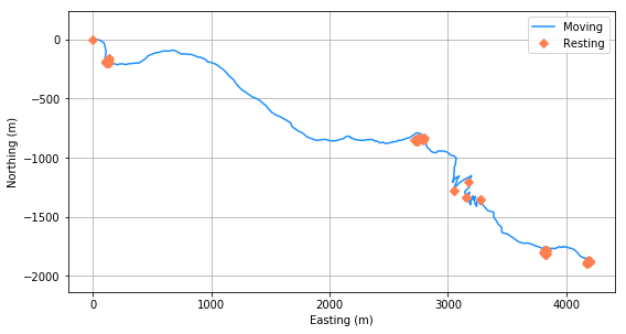

The last stop was when we reached our camp for the day near (4200, -1900). There are some scattered stops at the switchbacks near (3200, -1300). I did occasionally stop for pictures here or to catch my breath. I also hypothesize that switchbacks can cause a lower distance between successive track points, resulting in miss-classification of some moving points as stationary points.

Read the Details

Likelihood function for GPS movement data, normal inter-measurement times: Paper, model and likelihood function derivation for GPS movement detection.
Note: Convolution of a non-central chi-square with a central chi-square distribution: Paper, derivation of convolution integral for the probability density of the sum of a non-central chi-square and central chi-square variable
Likelihood function for GPS movement data (normal inter-measurement time distributions): Export of Jupyter Notebook, tools for computing and plotting maximum likelihood estimators for GPS movement detection.
Convolution of a non-central chi-square with a central chi-square distribution: Export of Jupyter Notebook, code and tests for numerical integration of the non-central and central chi-square convolution integral

Fred Ahrens,
CSEP Certified Systems Engineering Professional